
Molecular Docking vs Molecular Dynamics: What’s the Difference, and Do You Need Both?
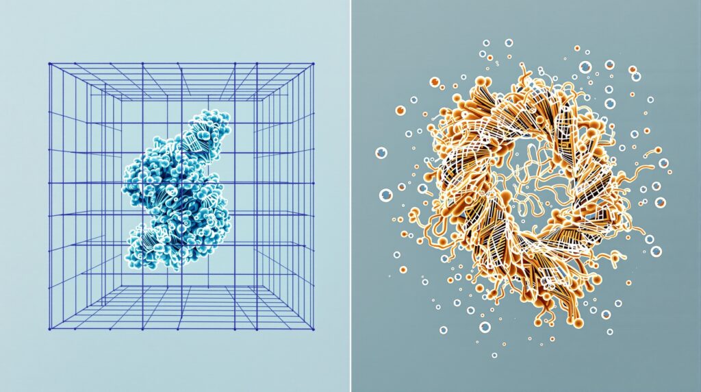
Molecular docking predicts where a ligand sits in a binding site and ranks candidate poses with a fast scoring function. Molecular dynamics then moves that complex through time in explicit solvent to test whether the pose survives. Docking generates the hypothesis, MD tests it. A defensible project usually needs both, in that order.
Students meet these two methods as a choice, usually because a supervisor said “do some docking” or “run a simulation” and left it there. They are not alternatives. They answer different questions, cost different amounts of computer time, and fail in different ways. This guide from the StemSkills Lab team (10+ years in sequence and structural bioinformatics, drug discovery and design, and multiscale molecular modeling) sets out exactly where one ends and the other begins, so you know which skill to learn first instead of picking at random. It sits inside our computational biology skills roadmap.
What is molecular docking actually predicting?
Docking predicts a pose: the position, orientation and conformation a ligand is likely to adopt inside a defined binding site, plus a number that ranks that pose against the alternatives. As the review by Salmaso and Moro puts it, docking has two parts, “an engine for conformations/orientations sampling and a scoring function, which associates a score to each predicted pose” (Salmaso & Moro, Frontiers in Pharmacology, 2018).
Two simplifications make that fast. The receptor is usually held rigid, so the protein cannot rearrange around the ligand. And there is no explicit solvent, so the water that really fills a binding pocket is approximated inside the scoring function rather than modelled molecule by molecule. Those two choices are why you can screen thousands of compounds, and they are also the source of almost every criticism of docking.
The tool’s own developers are direct about it. The official AutoDock Vina documentation states in its FAQ: Docking is an approximate approach.
(AutoDock Vina documentation, FAQ). That is not a disclaimer to skip past. It defines what your result is allowed to claim.
What does a docking score actually mean?
It means a ranking, not a measured binding affinity. The distinction matters because the units look convincing.
Take the numbers from the canonical Vina paper, Trott and Olson’s “AutoDock Vina: improving the speed and accuracy of docking with a new scoring function, efficient optimization, and multithreading” (Journal of Computational Chemistry, 2010, 31(2):455-461). On the 116 test complexes outside its training data, Vina reproduced the correct binding mode in 80% of cases against 53% for AutoDock 4, using the standard test that “the RMSD cutoff of 2 Angstrom is often used as a criterion of the correct bound structure prediction.” Good pose prediction. On the affinity side, the same paper reports a standard error of 2.75 kcal/mol for those 116 complexes.
Read those two figures together and the practical rule follows. Docking is reasonably good at telling you where a ligand binds and poor at telling you how strongly. Reporting that compound A scored -9.2 and compound B scored -8.7, and concluding that A is the better binder, sits well inside the method’s own error bar. This is the single most common way a docking chapter falls apart in a viva.
What is molecular dynamics, and what does it add that docking cannot?
MD integrates Newton’s equations of motion for every atom in the system, including the water. Nothing is held rigid, so the protein breathes, side chains rotate, waters enter and leave the pocket, and the ligand is free to shift or leave entirely.
That freedom is what makes MD a test rather than a prediction. A study on post-docking refinement states the benefit plainly: the approach “has the advantage of considering both the protein flexibility and the explicit treatment of solvent, which are usually neglected in most docking calculations” (Menin et al., International Journal of Molecular Sciences, 2023). Protein flexibility and explicit solvent are precisely the two things docking traded away for speed. MD buys them back and charges you in computer time.
The cost comes from the timestep. Hollingsworth and Dror’s review explains why: “To ensure numerical stability, the time steps in an MD simulation must be short, typically only a few femtoseconds each. Most of the events of biochemical interest, for example, functionally important structural changes in proteins, take place on timescales of nanoseconds, microseconds, or longer. A typical simulation thus involves millions or billions of time steps” (Hollingsworth & Dror, Neuron, 2018). You are stepping through femtoseconds to reach nanoseconds. That is a million steps per nanosecond.
Molecular docking vs molecular dynamics: how do they compare?
| Dimension | Molecular docking | Molecular dynamics |
|---|---|---|
| Question it answers | Where might this ligand bind, and in what orientation? | Does that arrangement hold up over time in a realistic environment? |
| Receptor treatment | Usually rigid | Fully flexible |
| Solvent | Implicit, folded into the scoring function | Explicit water molecules, simulated individually |
| Output | Ranked poses plus a score in kcal/mol | A trajectory: coordinates over time |
| Main metric | Score, and RMSD to a reference pose | RMSD over time, RMSF, hydrogen-bond occupancy, radius of gyration |
| Throughput | Thousands of ligands is routine | One complex at a time |
| Typical scale | Minutes per ligand | Days per system for useful sampling |
| Honest claim | “This pose is plausible and ranks above the alternatives” | “This pose stayed intact under these conditions for this long” |
Want the guided, hands-on version?
Our live Molecular Modeling & MD Simulations cohort bootcamp takes you from zero to running real docking and MD workflows, with a portfolio project for your grad-school applications.
How much longer does MD take than docking?
Different enough that it changes what you can attempt in a two-semester project.
For docking, the reference point is the Vina benchmark itself. Across 190 receptor-ligand complexes, “the average time was 1.16 minutes per complex,” measured on machines with two quad-core 2.66 GHz Xeon processors (Trott & Olson, 2010). That hardware is from 2010, so treat the figure as an order of magnitude rather than a prediction for your laptop. The paper also records where the speed comes from: Vina ran the benchmark 62 times faster than AutoDock in single-threaded mode, and 7.25 times faster again when using all 8 cores.
For MD, Hollingsworth and Dror give the modern reference point: “For systems with about 50,000 atoms (typical for a moderately sized, solvated protein), one GPU can currently simulate a microsecond in a few days.” Scale that down and a 100 ns production run on a solvated protein-ligand complex is a job of hours to days on a single decent GPU, not minutes.
So the ratio is roughly minutes against days, per ligand. That is the whole reason for the standard workflow: you dock many and simulate few.
Do you need both for a thesis project?
For a defensible one, usually yes, and the order is not negotiable. Docking narrows a library to a shortlist and produces starting coordinates. MD then asks whether those coordinates describe something real.
Salmaso and Moro describe MD in exactly this supporting role, noting it “can be used to assess stability, to refine and to rescore docking poses.” The empirical version of the question was tested directly by Sakano et al. (Biophysics and Physicobiology, 2016), who ran MD on docked poses and found that MD simulation provides useful information to complement the docking prediction, with some poses moving substantially once the protein and solvent were free to respond.
The practical test is ligand RMSD over the trajectory. The widely used GROMACS protein-ligand tutorial by Justin Lemkul explains the measurement: “the overall rotation and translation of the protein is removed via fitting and the RMSD reported is how much the [ligand] position has varied relative to the protein, which is a good indicator of how well the binding pose was preserved during the simulation” (GROMACS Tutorial 3, Step Nine). The command in that tutorial is:
gmx rms -s em.tpr -f md_0_10_center.xtc -n index.ndx -tu ns -o rmsd_jz4.xvg
And its expected result gives you a feel for what “stable” looks like: “The calculated RMSD should be about 0.15 ± 0.06 nm (1.5 ± 0.6 Angstrom), indicating only a very small change in the ligand’s position.” Note how neatly that lines up with the 2 Angstrom criterion docking uses to call a pose correct. A ligand that stays inside roughly 2 Angstrom of where you docked it has passed a meaningful test. One that drifts to 8 Angstrom and leaves the pocket has told you the docking result was an artefact, which is a genuine finding worth writing up.
One warning before you over-claim from a short run. As Menin et al. point out, “the short timescale that is used for most applications (tens of nanoseconds) is insufficient to sample the unbinding event for most poses, flattening the difference between the native pose and wrong but stable enough decoys.” A 10 ns simulation where the ligand stays put is weak evidence. It is a filter, not a proof.
What comes after MD if you want an actual binding affinity?
Neither method above gives you one directly, and the Lemkul tutorial is blunt about the trap students fall into when they extract an interaction energy from a trajectory. That quantity, it warns, “is NOT a free energy or a binding energy. In fact, most force fields are not parametrized in such a way that this quantity is actually physically meaningful.”
Two families of methods exist for the real calculation, and they sit at different points on the cost curve:
- End-state methods (MM/PBSA, MM/GBSA). Run on frames from your existing trajectory, so the marginal cost is low. The standard reference is Genheden and Ryde’s review, “The MM/PBSA and MM/GBSA methods to estimate ligand-binding affinities” (Expert Opinion on Drug Discovery, 2015). For GROMACS users the common implementation is gmx_MMPBSA, described by its authors as “a new tool based on AMBER’s MMPBSA.py aiming to perform end-state free energy calculations with GROMACS files.”
- Alchemical methods (FEP, thermodynamic integration). The rigorous option, and the expensive one. A large 2023 assessment of relative binding free energy predictions found that “in all 13,732 FEP+ relative binding free energy predictions, 57.5% were within 1 kcal/mol of the experimental value and 12.9% differed by more than 2 kcal/mol” (Ross et al., Communications Chemistry, 2023). Hollingsworth and Dror add the caveat: these methods “are computationally expensive, however, and generally only reliable when computing relative binding energies between ligands that share a similar scaffold.”
For most MSc projects, docking plus MD plus MM/PBSA is the realistic ceiling, and it is a perfectly respectable one as long as you state the error properties of each step.
Which one should you learn first?
Docking, without much doubt. It runs on hardware you already own, the feedback loop is minutes rather than days, and it forces you to learn the parts that MD also depends on: reading a PDB entry critically, adding hydrogens, assigning protonation states, defining a binding site, and validating your setup by redocking a co-crystallised ligand.
Learn MD second, once you have a pose worth defending. The concepts that trip people up in MD, force fields, solvation boxes, ions, energy minimisation, equilibration under NVT and NPT before production, are easier to absorb when you already have a specific complex you care about on your screen. Our pillar guides walk each path separately: learning molecular docking and learning molecular dynamics with GROMACS.
Frequently asked questions
Is a Vina binding affinity score the same as a binding free energy?
No. It is a scoring-function output in kcal/mol units intended for ranking. Trott and Olson report a standard error of 2.75 kcal/mol on their 116 held-out complexes, so small differences between compounds are not meaningful. Treat scores as a sort order, not a measurement.
How long should an MD simulation be to validate a docking pose?
There is no universal number, and the honest answer depends on what you are claiming. Published tutorials commonly use 10 ns for teaching, and research on pose validation notes that runs of tens of nanoseconds cannot sample unbinding. Longer is better, replicates are better still, and you should always report the length and the number of independent runs.
Can I skip docking and go straight to MD?
Only if you already have the bound complex, for example a co-crystallised structure from the PDB. MD does not search a binding site for you. Without a starting pose there is nothing for the simulation to test, and blind binding-site discovery by unbiased MD is far beyond typical project budgets.
Which is more accurate, docking or MD?
They are accurate about different things. Docking is good at generating a plausible pose and weak at affinity. MD is better at describing stability, flexibility and solvation, and it still depends entirely on the quality of the force field and the starting structure you gave it. Neither is a substitute for experimental validation.
Do I need a GPU to run either of these?
Docking with AutoDock Vina runs on an ordinary multi-core laptop; the official documentation lists no GPU requirement. MD is where a CUDA-capable GPU changes the timescale of your project from impractical to routine. Free GPU sessions on cloud notebooks and institutional HPC accounts are both viable routes if you do not own one.
Want the guided, hands-on version?
Our live Molecular Modeling & MD Simulations cohort bootcamp takes you from zero to running real docking and MD workflows, with a portfolio project for your grad-school applications.