
Covalent Docking Tutorial: Dock a Covalent Inhibitor
You cannot dock a covalent inhibitor with standard AutoDock Vina, whose own documentation lists covalent docking as planned functionality. Use AutoDock4’s flexible side chain method, which reproduced the crystal pose in 15 of 20 benchmark complexes, or run the free ADFR suite, which handles a covalent run in two commands.
This guide is part of our molecular docking pillar and our computational biology skills roadmap, written by the StemSkills Lab team, who have spent more than 10 years in sequence and structural bioinformatics, drug discovery and design, and multiscale molecular modeling.
Covalent inhibitors are a large part of modern drug discovery, and students are routinely asked to model one with the docking workflow they already know. That workflow does not apply. Every command, flag and version below was read off the official documentation on 6 October 2026, and the structure used in the walkthrough was checked against its Protein Data Bank entry on the same day.
Why can you not use AutoDock Vina for covalent docking?
Because Vina has no mechanism for forming a bond between the ligand and a receptor residue. Vina treats the ligand as a separate molecule exploring a grid. A covalent complex is one molecule, and the attachment point is fixed by chemistry rather than found by search.
The Vina documentation says so itself. Its frequently asked questions page lists the ability to “model covalent docking” among functionality planned for the future, alongside user-defined atom types and directional interaction models. The current release is v1.2.7, published in February 2025, and it does not include that mode. The Vina documentation instead points readers to Meeko, the Forli lab package, for covalent and reactive docking protocols.
This matters for a practical reason. A student who sets a grid box around a cysteine and runs Vina gets output: poses, affinities in kcal/mol, a ranked list. Nothing warns them that the ligand is sitting near the residue rather than bonded to it. The numbers look like docking results and are not covalent docking results. If you have been following our AutoDock Vina tutorial or our guide to setting the grid box, this is the point where the path diverges.
How do you identify the reactive residue and the warhead?
Covalent docking needs two facts before any software runs: which receptor residue forms the bond, and which ligand atom attacks it. Neither is predicted by the docking program. You supply both.
Cysteine is the usual target, because its thiol is nucleophilic at physiological pH. Serine, lysine, threonine and histidine also appear as covalent attachment points, and the AutoDock covalent methods can model the commonly modified residues. Establish the residue from the literature or from a crystal structure of a related complex, and never from a guess. If a crystal structure of your target with any covalent ligand exists, read the residue number off that entry.
The warhead is the reactive group on the ligand: acrylamides, chloroacetamides, nitriles, epoxides and boronic acids are common classes. Here is the limit students most often miss. Docking models the bound state. It does not predict whether your warhead will react with that residue, how fast, or whether the reaction is reversible. Reactivity and kinetics are chemistry questions, and a docking score cannot answer them. State that limit in your write-up rather than letting a reader infer that a good pose implies a good inhibitor.
Which free covalent docking route should you choose?
Four free routes exist, and they differ mainly in whether you need a GPU and how much published evidence supports them. The success rates below come from one benchmark, described in the next section, so compare them only against each other.
| Route | Cost | Hardware | Published success rate | Inputs you need | Beginner difficulty | Defensible in a methods section? |
|---|---|---|---|---|---|---|
| AutoDock4 flexible side chain | Free | CPU | 15 of 20 complexes, 75% | Receptor PDBQT, ligand joined to the residue side chain | Moderate; MGLTools preparation is the hurdle | Yes, with the Bianco 2016 citation |
| AutoDock4 two-point attractor | Free | CPU | 4 of 20 complexes, 20% | Receptor PDBQT, free ligand plus a custom potential | Moderate | Rarely; the same paper shows it performs poorly |
| ADFR covalent | Free | CPU | Not separately benchmarked; same flexible side chain principle | Receptor PDBQT, randomised ligand PDBQT, three atom serial numbers | Lowest; two commands once files are ready | Yes, with the ADFR citation |
| Meeko tethered plus AutoDock-GPU | Free | GPU, or Colab | Not separately benchmarked; implements the same two methods | Ligand SMILES, protonated receptor PDB, a SMARTS tether pattern | Highest; longest tool chain | Yes, and it is the current maintained route |
| DOCKovalent | Free web server | None, hosted | Not comparable; different method and benchmark | Receptor, residue, and a library in the server’s format | Low to run, high to interpret | Yes, with the London 2014 citation |
| Commercial (CovDock, FITTED, ICM) | Paid licence | Varies | Vendor reported, not compared here | Varies by package | Low, graphical interfaces | Yes, if you have the licence |
For a first covalent docking job on a normal laptop, ADFR is the route to pick. It runs on CPU, its covalent tutorial is published with working data files, and the whole run is two commands. Choose Meeko with AutoDock-GPU when you have GPU access and want the actively maintained chain. Note that the Meeko documented route runs on AutoDock-GPU, not Vina, so a machine with no GPU means Colab or a different route.
What does the benchmark actually say about accuracy?
One paper underpins both AutoDock covalent methods, and its numbers are specific enough to make your choice for you. Bianco, Forli, Goodsell and Olson applied both methods to a training set of 20 diverse protein-ligand covalent complexes and measured the RMSD between the lowest energy pose and the experimental coordinates, counting a result under 3.0 angstroms as successful.
The flexible side chain method reproduced the experimental coordinates in 15 of 20 systems, a 75% success rate. The two-point attractor method managed 4 of 20, a 20% success rate (Bianco G, Forli S, Goodsell DS, Olson AJ, Protein Science 2016;25(1):295-301). The paper explains the gap: in the flexible side chain method the ligand is aligned along the C-alpha to C-beta bond and only torsions need searching, while the two-point attractor method docks the ligand untethered and carries far more degrees of freedom.
There is a second finding worth knowing before you commit to a large ligand. The flexible side chain method’s accuracy falls with ligand flexibility, and the authors report only one successful result for ligands with more than nine torsional degrees of freedom. If your compound is large and floppy, expect the method to struggle and say so in your discussion. The AutoDock covalent docking resource page hosts the tutorial and script files for the flexible residue method and asks users to cite this paper.
Want the guided, hands-on version?
Our live Molecular Modeling & MD Simulations cohort bootcamp takes you from zero to running real docking and MD workflows, with a portfolio project for your grad-school applications.
How do you run a covalent docking job in ADFR, step by step?
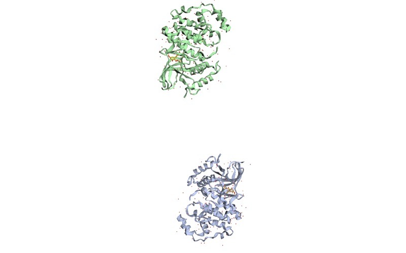
The official ADFR covalent docking tutorial re-docks the native covalent ligand of PDB entry 3C9W, and it is the clearest worked example available for free. That entry is the crystal structure of ERK-2, listed in the Protein Data Bank as mitogen-activated protein kinase 1, with the natural product hypothemycin covalently bound, solved by X-ray diffraction at 2.50 angstrom resolution and containing two protein chains, A and B. The ligand carries the three-letter code HMY, and the file records the bond explicitly: a LINK record joins atom C11 of HMY to the SG atom of CYS 164 in chain A at a distance of 1.62 angstroms. That LINK record is where the two atom numbers in the command below come from.
Install ADFRsuite first. The current release is ADFRsuite 1.0 rc1, which contains ADFR v1.2 and AGFR v1.2, available from the ADFR downloads page.
Step 1. Build the covalent target file with AGFR. The receptor and the covalent ligand must share three atoms: two that form the bond and one anchor atom on the receptor side that defines the torsion. The tutorial’s command is:
agfr -r data/3c9w.pdbqt -b user 28.565 6.329 6.985 22.5 22.5 22.5 -c 1593 1596 -t 1591 -x A:CYS164 -o 3c9w_cov_cmdlineEach flag earns its place:
-cor--covalentBondtakes the PDB serial numbers of the two receptor atoms that form the bond, as they appear in the PDBQT file.-tor--covalentBondTorsionAtomtakes the third atom, used to compute the torsion angle of the covalent bond.-xor--covalentResidueslimits how far AGFR walks the receptor. Leave it out on this example and the spurious bond the ligand makes with the receptor causes AGFR to cut out in excess of 1600 atoms when it works out which atoms to remove for the affinity maps.-b userplaces the box manually from the six numbers that follow, three for the centre and three for the size. This is the only box mode for which padding is ignored.-onames the output target, here3c9w_cov_cmdline.trg.
The box centre, the box size and the three serial numbers are specific to the tutorial’s own 3c9w.pdbqt. Do not copy them onto your own receptor. Open your file, find the two atoms of your bond and the anchor atom, and read your own serial numbers from it.
Step 2. Dock the randomised ligand.
adfr -l data/3c9w_ligandWithSideChain_random.pdbqt -t 3c9w_cov_cmdline.trg --jobName covalent -C 1 2 3 --nbRuns 8 --maxEvals 100000 -O --seed 1The ligand file is the native ligand with its conformation, position and orientation randomised, which is what makes this a genuine test rather than a replay. The tutorial sets --nbRuns 8 and --maxEvals 100000 for speed; ADFR’s own defaults are 50 searches of 2.5 million evaluations each, and a real docking problem wants something closer to the defaults. --seed fixes the random number generator so the run can be reproduced, which matters for the same reasons covered in our guide to exhaustiveness and reproducible docking.
The run writes three files: a _summary.dlg log, a _out.pdbqt containing the poses, and a .dro docking object holding the inputs, outputs and metadata. One detail from the tutorial explains why no translational sampling appears in the setup: no translational points are needed, because the covalent bond already positions the ligand in the box. The method is described in Ravindranath PA, Forli S, Goodsell DS, Olson AJ, Sanner MF, PLoS Computational Biology 2015;11(12):e1004586.
How does the Meeko and AutoDock-GPU tethered route work?
Meeko is the maintained modern route, currently at v0.8.0, and its tethered docking tutorial reproduces a covalent intermediate: adenosine monophosphate attached to the catalytic histidine of a bacterial RNA 3′ cyclase, PDB entry 3KGD, as the conjugate named HIE_AMP. The chain has more steps than ADFR, and each one has a purpose.
- Build the conjugate.
scrub.pyturns a SMILES string for the ligand-plus-side-chain conjugate into a 3D conformer with explicit hydrogens. The conjugate must contain the flexible ligand part, the flexible side chain part, and the residue’s C-alpha and C-beta, which act as the two fixed attractor points. - Protonate the receptor.
reduce2.pyadds and optimises hydrogens. The tutorial notes that the CRYST1 card from the original PDB file has to be combined into the input, a requirement of the reduce2 version current as of October 2024. - Prepare the receptor.
mk_prepare_receptor.pywrites the rigid receptor PDBQT and the grid parameter file, using--default_altlocto pick an alternate location,-fto name the flexible residue,--box_envelopingwith--paddingto place the box, and-jto emit a receptor JSON file you will want later for PDB export. - Prepare the tethered ligand.
mk_prepare_ligand.pytakes--receptor,--rec_residuein chain:residue:number form, and a--tether_smartspattern with one-based--tether_smarts_indicesthat locate the two attractor atoms. In the tutorial these are"A:HIS:309", the pattern"n1cc(CC)nc1"and indices"5 4". - Compute maps and dock. Run
autogrid4 -pon the grid parameter file, then run AutoDock-GPU. The step that surprises people: tethered docking does not take a ligand file at all. There is no-Lor--lfile. The ligand travels inside the flexible side chain file, passed with-For--flexres. - Export the poses.
mk_export.pyconverts the DLG output to SDF, and the-koption keeps the covalent ligand that is being treated as a flexible residue.
AutoDock-GPU is at v1.6. If you are on a Mac without a suitable GPU, our notes on running GROMACS and AutoDock Vina on Apple Silicon explain the constraints, and the tutorial’s Colab examples are the practical answer.
How do you validate a covalent docking result?
The defensible validation move is a redock. Take a crystal structure of your target with a known covalent ligand, randomise that ligand, dock it back, and report the RMSD to the experimental coordinates. That is precisely the protocol the published benchmark uses, and the 3.0 angstrom threshold gives you a stated criterion rather than an opinion.
Two reporting rules follow from how covalent docking works.
First, a covalent docking score is not comparable to a Vina affinity. The energy reported for a tethered run describes a different physical situation, with the ligand bonded and much of its translational freedom removed. Never place covalent scores and non-covalent Vina affinities in one ranked table, and never present either as a binding affinity. Our guide to interpreting docking results covers what a score can and cannot support.
Second, report the interactions, not only the number. Once you have a pose, the useful output is the contact map around the attachment point, which you can produce with the tools in our guide to protein-ligand interaction diagrams. When you write it up, name the method, the residue, the warhead, the redock RMSD and the software version, following our guide to writing a docking methods section. If the covalent complex is heading into simulation, our protein-ligand MD tutorial in GROMACS is the next step, with the caveat that a covalent bond needs correct topology rather than a standard ligand parameterisation.
Troubleshooting: real failures and what to do about them
You picked the wrong two atom serial numbers and the bond formed to the backbone. The serial numbers in -c refer to atoms in your PDBQT file, not to the original PDB and not to residue numbers. For a cysteine attachment the receptor-side atom is normally the side chain sulfur, SG, not N, CA or C. Open the PDBQT, find the atom by name, and use that line’s serial number.
AGFR cut an enormous piece out of your receptor. You omitted -x or --covalentResidues. Residue traversal followed a spurious bond and removed far more of the protein than intended. Restrict traversal to the covalent residue, as the tutorial does with -x A:CYS164.
Your ADFR covalent run reproduces the input pose suspiciously well. Check that you randomised the ligand. The tutorial’s ligand file is explicitly randomised in conformation, position and orientation. Docking an un-randomised native ligand back into its own site tests nothing and will not survive review.
PDBQT preparation fails because MGLTools needs Python 2. This is the most common blocker on the AutoDock4 route. Use the Meeko scripts for preparation instead, which are current Python, or follow the preparation route in our guide to preparing a protein and ligand for docking.
Your SMARTS tether matches more than one site in the ligand. Then the indices point at the wrong atoms and the tether is built in the wrong place. Test the pattern against your molecule and confirm it matches exactly once. Remember the indices are one-based.
You centred the grid box as if this were an ordinary docking run. For a covalent run the ligand position is set by the bond, so the box only has to enclose the region the tethered ligand can reach. Over-sizing the box wastes map computation without improving sampling, and no translational sampling is being done in any case.
You reused grid maps from the reactive docking tutorial. The Meeko documentation warns against exactly this. The reactive tutorial’s grid parameter file carries extra parameters, so its maps cannot be reused for a tethered run even though the filenames and commands look alike.
Frequently asked questions
Can AutoDock Vina do covalent docking at all?
No. Vina’s documentation lists covalent docking among functionality planned for the future, and release v1.2.7 does not implement it. Use AutoDock4, ADFR or Meeko with AutoDock-GPU. If you want the differences between the two AutoDock engines, see our Vina versus AutoDock4 comparison.
Which free covalent docking method is most accurate?
The flexible side chain method, on the only direct comparison published. It reproduced the crystal pose in 15 of 20 benchmark complexes against 4 of 20 for the two-point attractor method, using a 3.0 angstrom success threshold. Both are described in the same 2016 Protein Science paper.
Do I need a GPU for covalent docking?
Not for AutoDock4 or ADFR, which run on CPU. The Meeko tethered workflow is documented against AutoDock-GPU, so that route needs a suitable GPU or a Colab notebook. Start with ADFR if you only have a laptop.
Does covalent docking predict whether my compound will react?
No. Docking models the bound state after the bond exists. It says nothing about reaction rate, reversibility or warhead selectivity. Those need chemistry and experimental data, and claiming otherwise from a docking score is the most common overstatement in covalent modelling write-ups.
Can I compare a covalent docking score with a Vina binding affinity?
No. The two numbers describe different physical situations, and the covalent run removes most of the ligand’s translational freedom. Never rank them in one table. Report covalent results against other covalent results, and validate with a redock RMSD instead.
Which residues can be modelled as covalent attachment points?
Cysteine is the most common, and the AutoDock covalent methods also handle other frequently modified residues including serine, lysine, threonine and histidine. The ADFR tutorial uses a cysteine and the Meeko tutorial uses a histidine. Confirm your residue from literature or a crystal structure.
The short version: pick the route your hardware supports, supply the residue and the attachment atoms yourself rather than expecting software to find them, redock a known complex to earn the right to trust your protocol, and keep covalent scores in their own table. A covalent docking result that names its method, its residue and its redock RMSD will hold up. One presented as a binding affinity will not.
Want the guided, hands-on version?
Our live Molecular Modeling & MD Simulations cohort bootcamp takes you from zero to running real docking and MD workflows, with a portfolio project for your grad-school applications.